MLE Example

In the previous example you looked at a robot taking repeated measurements of the same feature in the environment. This example demonstrated the fundamentals of maximum likelihood estimation, but was very limited since it was only estimating one parameter - z_1 .

In this example, you will have the opportunity to get hands-on with a more complicated 1-dimensional estimation problem.

Motion and Measurement Example

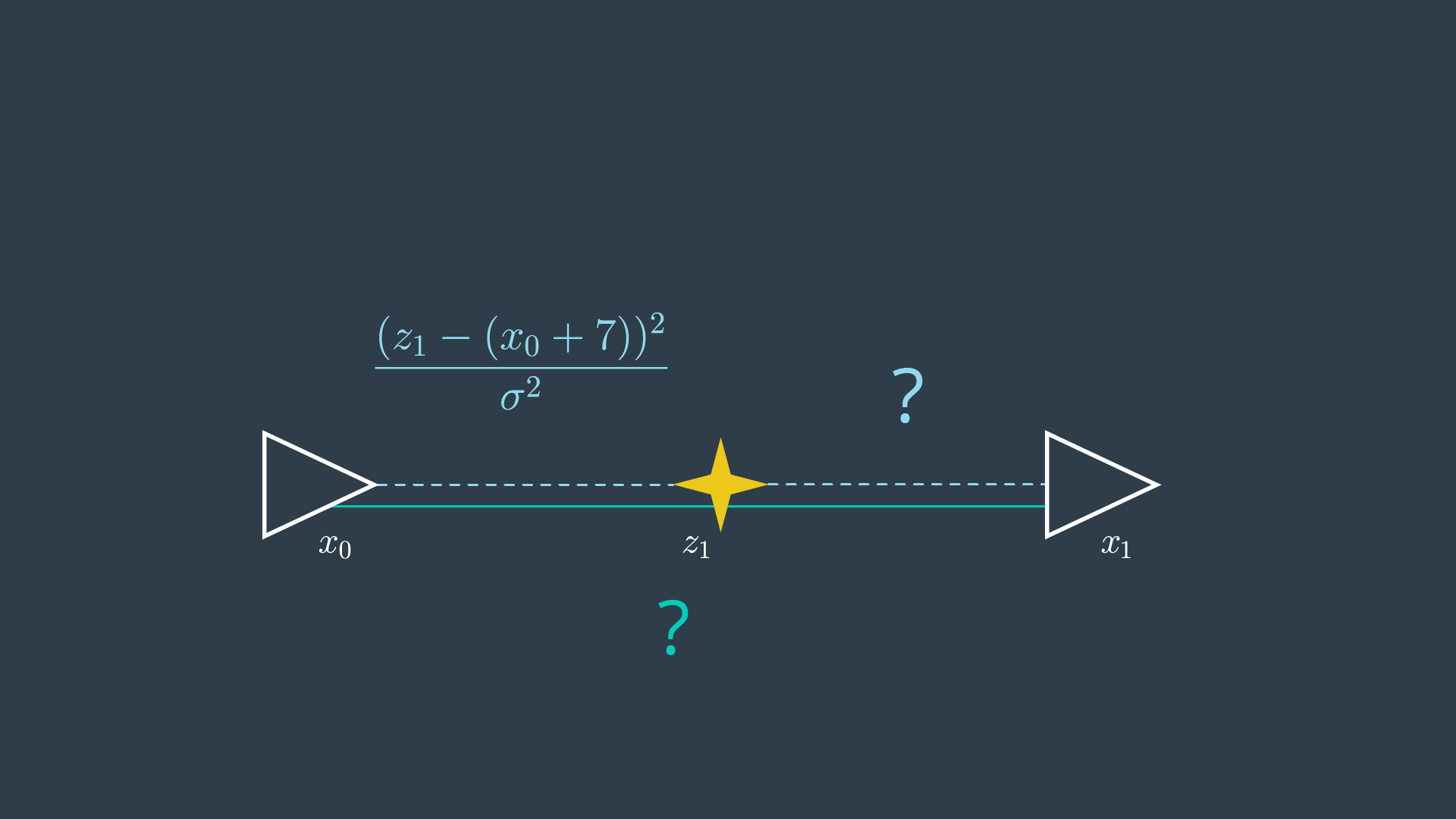
The robot starts at an arbitrary location that will be labeled 0, and then proceeds to measure a feature in front of it - the sensor reads that the feature is 7 meters way. The resultant graph is shown in the image below.

After taking its first measurement, the following Gaussian distribution describes the robot’s most likely location. The distribution is highest when the two poses are 3 metres apart.

p(x)=\frac{1}{\sigma\sqrt{2\pi}}e^{-\frac{(z_1-(x_0 + 7))^2}{2\sigma^2}}

Recall that since we constrained the robot’s initial location to 0, x_0 can actually be removed from the equation.

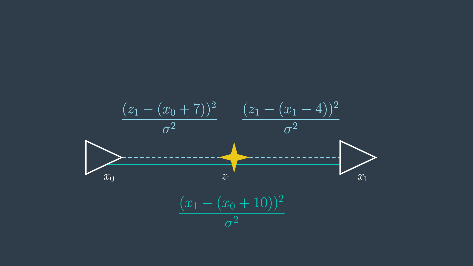
Next, the robot moves forward by what it records to be 10 meters, and takes another measurement of the same feature. This time, the feature is read to be 4 meters behind the robot. The resultant graph looks like so,

Now it’s up to you to determine what the two new constraints look like!

Constraints Quizzes

Which of the following is the correct constraint for the robot’s motion from x_0 to x_1 ?

\frac{(x_1 - (x_0 + 10))^2}{\sigma^2}

\frac{(x_1 - (x_0 - 10))^2}{\sigma^2}

\frac{(x_0 - (x_1 + 3))^2}{\sigma^2}

\frac{(x_1 - (x_0 - 3))^2}{\sigma^2}

SOLUTION:

\frac{(x_1 - (x_0 + 10))^2}{\sigma^2}

Which of the following is the correct constraint for the robot’s measurement from x_1 to z_1 ?

\frac{(x_1 - (z_1 - 3))^2}{\sigma^2}

\frac{(z_1 - (x_1 + 4))^2}{\sigma^2}

\frac{(z_1 - (x_1 + 3))^2}{\sigma^2}

\frac{(z_1 - (x_1 - 4))^2}{\sigma^2}

SOLUTION:

\frac{(z_1 - (x_1 - 4))^2}{\sigma^2}

Sum of Constraints

The completed graph, with all of its labelled constraints can be seen below.

Now, the task at hand is to minimize the sum of all constraints:

J_{GraphSLAM} = \frac{(z_1-7)^2}{\sigma^2} + \frac{(x_1 - (x_0 + 10))^2}{\sigma^2} + \frac{(z_1 - (x_1 - 4))^2}{\sigma^2}

To do this, you will need to take the first derivative of the function and set it to equal zero. Seems easy, but wait - there are two variables! You’ll have to take the derivative with respect to each, and then solve the system of equations to calculate the values of the variables.

For this calculation, assume that the measurements and motion have equal variance.

See if you can work through this yourself to find the values of the variables, but if you’re finding this task challenging and would like a hint, skip ahead to the solution to the quiz where I will step you through the process.

Optimization Quiz

What are the estimated locations of z_1 and x_1 based on your calculations?

z_1 = 6.5, x_1 = 10.5

z_1 = 7, x_1 = 11

z_1 = 6.5, x_1 = 10.75

z_1 = 6.67, x_1 = 10.33

SOLUTION:

z_1 = 6.67, x_1 = 10.33

If you’ve gotten this far, you’ve figured out that in the above example you needed to take the derivative of the error equation with respect to two different variables - z_1 and x_1 - and then perform variable elimination to calculate the most likely values for z_1 and x_1 . This process will only get more complicated and tedious as the graph grows.

Optimization with Non-Trivial Variances

To make matters a little bit more complicated, let’s actually take into consideration the variances of each measurement and motion. Turns out that our robot has the fanciest wheels on the market - they’re solid rubber (they won’t deflate at different rates) - with the most expensive encoders. But, it looks like the funds ran dry after the purchase of the wheels - the sensor is of very poor quality.

Redo your math with the following new information,

Motion variance: 0.02,
Measurement variance: 0.1.

Optimization Quiz 2

What are the estimated locations of z_1 and x_1 based on your calculations when taking into account the variances?

z_1 = 6.61, x_1 = 10.12

z_1 = 6.66, x_1 = 10.33

z_1 = 6.54, x_1 = 10.09

z_1 = 6.6, x_1 = 10.25

SOLUTION:

z_1 = 6.54, x_1 = 10.09

That seemed to be a fair bit more work than the first example! At this point, we just have three constraints - imagine how difficult this process would be if we had collected measurement and motion data over a period of half-an hour, as may happen when mapping a real-life environment. The calculations would be tedious - even for a computer!

Solving the system analytically has the advantage of finding the correct answer. However, doing so can be very computationally intensive - especially as you move into multi-dimensional problems with complex probability distributions. In this example, the steps were easy to perform, but it only takes a short stretch of the imagination to think of how complicated these steps can become in complex multidimensional problems.

Well, what is the alternative? you may ask. Finding the maximum value can be done in two ways - analytically and numerically . Solving the problem numerically allows for a solution to be found rather quickly, however its accuracy may be sub-optimal. Next, you will look at how to solve complicated MLE problems numerically.